When working with Excel, one of the most powerful tools at your disposal is the ability to format tables effectively. Proper table formatting not only enhances the visual appeal of your spreadsheets but also improves readability and understandability. In this article, we will delve into five essential tips for formatting tables in Excel, exploring both the basics and some advanced techniques to take your spreadsheet skills to the next level.
Understanding the Basics of Table Formatting

Before diving into the tips, it’s crucial to understand the basics of table formatting in Excel. This includes selecting the data range you wish to format, going to the “Insert” tab on the Ribbon, and then clicking on “Table.” Excel provides a variety of pre-designed table styles that can instantly enhance the appearance of your data. However, for more customized and professional-looking tables, you’ll want to explore further options.
Tip 1: Apply Conditional Formatting
Conditional formatting is a powerful tool in Excel that allows you to highlight cells based on specific conditions, such as values above or below a certain threshold. To apply conditional formatting to your table, select the data range, go to the “Home” tab, find the “Styles” group, and click on “Conditional Formatting.” From here, you can choose from a variety of rules, such as “Highlight Cells Rules,” “Top/Bottom Rules,” “Data Bars,” “Color Scales,” and “Icon Sets.” This feature can help draw attention to important trends or outliers within your data.
| Conditional Formatting Rule | Description |
|---|---|
| Highlight Cells Rules | Highlight cells based on values, formulas, or formatting. |
| Top/Bottom Rules | Highlight top or bottom values or percentages. |
| Data Bars | Display data bars in cells to compare values. |
| Color Scales | Apply color scales to display data distribution. |
| Icon Sets | Use icons to categorize and highlight data. |

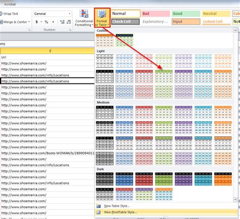
Tip 2: Utilize Table Styles
Excel offers a wide range of pre-designed table styles that can instantly improve the appearance of your tables. To apply a table style, select your table, go to the “Table Design” tab (which appears once you’ve created a table), and click on the style you prefer from the “Table Styles” group. You can also customize the style further by checking or unchecking the boxes for “Header Row,” “Total Row,” “First Column,” “Last Column,” “Banded Rows,” and “Banded Columns” to tailor the look to your needs.
Tip 3: Customize Your Table’s Appearance
Beyond the pre-designed styles, Excel allows you to customize almost every aspect of your table’s appearance. This includes changing the font, font size, and color of the text, as well as adjusting the background colors and borders of the cells. To customize, select the part of the table you wish to change, right-click, and choose “Format Cells” to access a wide range of formatting options.
Tip 4: Use Freezing Panes for Better Viewing
For larger datasets, navigating through the table can be cumbersome, especially when header rows or columns are out of view. Excel’s “Freeze Panes” feature solves this issue by allowing you to lock specific rows or columns in place as you scroll. To freeze panes, go to the “View” tab, click on “Freeze Panes,” and then choose whether you want to freeze the top row, the first column, or both, depending on your needs.
Tip 5: Protect Your Table
Finally, once you’ve formatted your table, you may want to protect it from accidental changes. Excel allows you to lock the entire worksheet or specific ranges within it. To protect your table, select the range you want to protect, right-click, and choose “Format Cells.” Then, in the “Protection” tab, check the “Locked” box. After doing this, you’ll need to protect the worksheet by going to the “Review” tab, clicking on “Protect Sheet,” and setting a password. This ensures that your carefully formatted table remains intact.
Key Points
- Apply conditional formatting to highlight important data trends.
- Utilize and customize table styles for a professional look.
- Customize the table's appearance for better readability.
- Use freezing panes for easier navigation of large datasets.
- Protect your table from accidental changes by locking cells and protecting the worksheet.
In conclusion, formatting tables in Excel is not just about making your spreadsheets look good; it's about presenting your data in a clear, understandable, and actionable way. By applying these five tips, you can significantly enhance your ability to communicate insights and trends within your data, making you more effective in your work or studies.
How do I apply a table style in Excel?
+To apply a table style, select your table, go to the “Table Design” tab, and click on the style you prefer from the “Table Styles” group.
What is conditional formatting used for?
+Conditional formatting is used to highlight cells based on specific conditions, such as values above or below a certain threshold, to draw attention to important trends or outliers within your data.
How can I protect my table from accidental changes?
+To protect your table, select the range you want to protect, right-click, and choose “Format Cells.” Then, in the “Protection” tab, check the “Locked” box. After doing this, protect the worksheet by going to the “Review” tab, clicking on “Protect Sheet,” and setting a password.