Excel is a powerful tool for data analysis and manipulation, and one of its most useful features is the IF function, which allows users to make decisions based on specific conditions. The IF function is often used in conjunction with other functions, such as AND, OR, and NOT, to create complex conditional statements. In this article, we will explore five essential Excel IF Then tips to help you master this powerful function and take your data analysis to the next level.
Key Points
- Using the IF function to make simple decisions based on a condition
- Nesting IF functions to create complex conditional statements
- Using the IFERROR function to handle errors and exceptions
- Applying conditional formatting with IF functions
- Using IF functions with other functions, such as AND and OR, to create advanced conditional statements
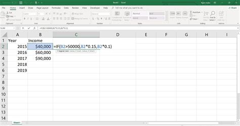
Tip 1: Using the IF Function to Make Simple Decisions

The IF function is used to make a decision based on a condition. The syntax of the IF function is: IF(logical_test, [value_if_true], [value_if_false]). The logical_test is the condition that you want to test, value_if_true is the value that is returned if the condition is true, and value_if_false is the value that is returned if the condition is false. For example, if you want to determine whether a student has passed or failed a test based on their score, you can use the IF function as follows: =IF(A1>60, “Pass”, “Fail”). In this example, A1 is the cell that contains the student’s score, and the IF function returns “Pass” if the score is greater than 60 and “Fail” otherwise.
Example of Using the IF Function
Suppose you have a list of student scores in column A, and you want to determine whether each student has passed or failed a test. You can use the IF function to create a formula that returns “Pass” or “Fail” based on the score. The formula would be: =IF(A1>60, “Pass”, “Fail”). You can then copy this formula down to the other cells in the column to apply it to all the students.
| Student Score | Result |
|---|---|
| 70 | =IF(A2>60, "Pass", "Fail") returns "Pass" |
| 50 | =IF(A3>60, "Pass", "Fail") returns "Fail" |

Tip 2: Nesting IF Functions to Create Complex Conditional Statements

Nesting IF functions allows you to create complex conditional statements that can test multiple conditions. The syntax of a nested IF function is: IF(logical_test, IF(logical_test, [value_if_true], [value_if_false]), [value_if_false]). For example, if you want to determine whether a student has passed or failed a test based on their score, and also whether they have attended more than 80% of the classes, you can use a nested IF function as follows: =IF(A1>60, IF(B1>0.8, “Pass”, “Fail due to attendance”), “Fail”). In this example, A1 is the cell that contains the student’s score, and B1 is the cell that contains the student’s attendance percentage.
Example of Nesting IF Functions
Suppose you have a list of student scores and attendance percentages in columns A and B, and you want to determine whether each student has passed or failed a test based on their score and attendance. You can use a nested IF function to create a formula that returns “Pass”, “Fail due to attendance”, or “Fail” based on the score and attendance. The formula would be: =IF(A1>60, IF(B1>0.8, “Pass”, “Fail due to attendance”), “Fail”). You can then copy this formula down to the other cells in the column to apply it to all the students.
Tip 3: Using the IFERROR Function to Handle Errors and Exceptions
The IFERROR function is used to handle errors and exceptions that may occur when using the IF function. The syntax of the IFERROR function is: IFERROR(cell, value_if_error). The cell is the cell that contains the formula that may return an error, and value_if_error is the value that is returned if an error occurs. For example, if you want to divide two numbers and return a custom error message if the denominator is zero, you can use the IFERROR function as follows: =IFERROR(A1/B1, “Cannot divide by zero”).
Example of Using the IFERROR Function
Suppose you have a list of numbers in column A, and you want to divide each number by a value in column B. You can use the IFERROR function to handle errors that may occur if the denominator is zero. The formula would be: =IFERROR(A1/B1, “Cannot divide by zero”). You can then copy this formula down to the other cells in the column to apply it to all the numbers.
Tip 4: Applying Conditional Formatting with IF Functions
Conditional formatting allows you to highlight cells based on specific conditions. You can use IF functions to create conditional formatting rules that highlight cells based on complex conditions. For example, if you want to highlight cells that contain values greater than 60, you can use the IF function as follows: =IF(A1>60, TRUE, FALSE). You can then apply this formula to a conditional formatting rule to highlight the cells that meet the condition.
Example of Applying Conditional Formatting with IF Functions
Suppose you have a list of numbers in column A, and you want to highlight the cells that contain values greater than 60. You can use the IF function to create a conditional formatting rule that highlights the cells that meet the condition. The formula would be: =IF(A1>60, TRUE, FALSE). You can then apply this formula to a conditional formatting rule to highlight the cells that contain values greater than 60.
Tip 5: Using IF Functions with Other Functions to Create Advanced Conditional Statements

IF functions can be used with other functions, such as AND and OR, to create advanced conditional statements. The AND function returns TRUE if all the conditions are true, while the OR function returns TRUE if at least one of the conditions is true. For example, if you want to determine whether a student has passed or failed a test based on their score and attendance, and also whether they have completed all the assignments, you can use the IF function with the AND function as follows: =IF(AND(A1>60, B1>0.8, C1=100), “Pass”, “Fail”). In this example, A1 is the cell that contains the student’s score, B1 is the cell that contains the student’s attendance percentage, and C1 is the cell that contains the student’s assignment completion percentage.
Example of Using IF Functions with Other Functions
Suppose you have a list of student scores, attendance percentages, and assignment completion percentages in columns A, B, and C, and you want to determine whether each student has passed or failed a test based on their score, attendance, and assignment completion. You can use the IF function with the AND function to create a formula that returns “Pass” or “Fail” based on the conditions. The formula would be: =IF(AND(A1>60, B1>0.8, C1=100), “Pass”, “Fail”). You can then copy this formula down to the other cells in the column to apply it to all the students.
What is the syntax of the IF function in Excel?
+The syntax of the IF function in Excel is: IF(logical_test, [value_if_true], [value_if_false]).
How do I nest IF functions in Excel?
+To nest IF functions in Excel, you can use the following syntax: IF(logical_test, IF(logical_test, [value_if_true], [value_if_false]), [value_if_false]).
What is the purpose of the IFERROR function in Excel?
+The IFERROR function in Excel is used to handle errors and exceptions that may occur when using the IF function.
In conclusion, the IF function is a powerful tool in Excel that allows you to make decisions based on specific conditions. By mastering the IF function and its various applications, you can create complex conditional statements, handle errors and exceptions, and apply conditional formatting to your data. Whether you are a beginner or an advanced user, these five Excel IF Then tips will help you to take your data analysis to the next level and make informed decisions based on your data.